The two dimensional algorithm has been implemented in Maple and run on some inputs including
for
The operations of the two dimensional
Zeros
and
Narrow
procedures are represented graphically in
Figures 5.1-5.2. Most rectangles represent regions of the
Finally,
Figures 6.1-6.2
are closeups for selected solutions of these two systems which picture the trajectories
of approximate solutions
and these lead to solution (x,y)=(2.8331478920493421425, 2.8331478920493421425) as shown in Figure 6.1. |
|
|
Results II
|

 for
for
 and
and
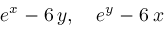
 for these examples. The solutions being sought are the intersection points of
these curves.
for these examples. The solutions being sought are the intersection points of
these curves.
 -plane eliminated by steps in either
Zeros
or
Narrow. Only the very smallest rectangles represent regions that have not been eliminated
and these surround the solutions we seek.
-plane eliminated by steps in either
Zeros
or
Narrow. Only the very smallest rectangles represent regions that have not been eliminated
and these surround the solutions we seek.
 computed by two dimensional versions of the
Locate
and
Newton
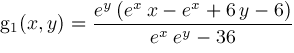
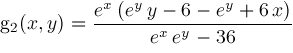
procedures. The Newton iteration formulas for example (1) are
computed by two dimensional versions of the
Locate
and
Newton
procedures. The Newton iteration formulas for example (1) are